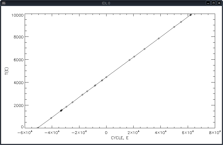
TIMING DATA The data has been taken from . All timing stamps are in BJD using the TDB time scale. No further transformations needed. A total of 42 timing measurements exist. However, Potter et al. have not included data points from Dai et al. (2010). See Potter et al. (2011) text for details. In this analysis I will consider the full set of timings as a start and as presented in Potter et al. (2011). LINEAR EPHEMERIS - FITTING A STRAIGHT LINE USING LINFIT In general I am using IDL for the timing analysis. The cycle or ephemeris numbers have been obtained from IDL> ROUND((BJDMIN-TZERO)/PERIOD) where BJDMIN are all 42 timing measurements, TZERO is an arbitrary timing measurement that defines the CYCLE=E=0 and PERIOD is the binary orbital period (0.087865425 days) and was taken from , Table 2. In this work I will use TZERO=BJD 2,450,021.779388. It is a bit different from the TZERO used in in order to introduce a bit variation and also because I think the center of mass of the data points is as chosen by me. As a first step I used IDL’s LINFIT code to fit a straight line with the MEASURE_ERROR keyword set to an array holding the timing measurements errors (Table 2, 3rd column, Potter et al. 2011). This way the square of deviations are weighted with 1/σ² where σ is the standard timing error for each timing measurement. This is standard procedure and was also used in Potter et al. (2011). The average or mean timing error for the 42 measurements is 6.0 seconds (the standard deviation is also 6.0 seconds) with 0.74 seconds as the smallest and 17 seconds as the largest error. Also I have rescaled the timing measurements by subtracting the first timing measurement from all the others. Rescaling introduces nothing spooky to the analysis and has the advantage to avoid dynamic range problems. This is in particular needed for a later analysis when using MPFIT. Using LINFIT the resulting reduced χ² value was 95.22 (χ² = 3808.82 with (42-2) degrees of freedom) with the ephemeris (or computed timings) given as T(E) = BJD~2450021.77890(6) + E \times 0.0878654291(1) The corresponding root-mean-square (RMS) scatter of the data around the best-fit line is 27.5 seconds and the corresponding standard deviation is 27.7 seconds. As expected they should both be similar. To measure scatter of data around any best-fit model, I will use the RMS quantity. The RMS scatter is 5 times the average timing error and could be indicative of a systematic process. As a test the CURVEFIT routine has been used in a similar manner. The resulting reduced chi2 was also 95.22 matching and confirming the result from the previous section. The /NODERIVATIVE keyword does not change anything and expressions for the partial derivative has been included. The RMS also agrees with the results obtained from LINFIT. However, the formal 1σ uncertainties in the best-fit parameters (TZERO and PERIOD) are one magnitude smaller compared to the equivalent values obtained from LINFIT. The data and the best-fit line (obtained from LINFIT) is shown in Fig. [linearfit] with the residuals plotted in Fig. [linearfit_res]. There is absolutely no difference when using the results from CURVEFIT. Linear ephemeris - conclusion After fitting a straight line and visually inspecting the residual plots I cannot see any convincing trend that should justify a quadratic ephemeris (linear + a quadratic term). What I see is a sinusoidal variation around the best-fit line. Relative to the linear line the first timing measurement arrives 20s earlier than expected. Then the trend goes down and increases again to 40s at E=0, then decreases again to a minimum to around 20s and increases again thereafter. There is no obvious quadratic trend from looking at the residuals in Fig. [linearfit_res]. QUADRATIC EPHEMERIS Although there is no obvious reason to include a quadratic term I will nevertheless consider a quadratic model. I will do this by again using IDL’s CURVEFIT procedure and the MPFIT package (also IDL) which is a more sophisticated fitting tool utilizing the Levenberg-Marquardt least-squares minimization algorithm developed by Marwardt. Quadratic ephemeris using CURVEFIT The results from CURVEFIT are surprising. The best-fit χ² value was 3718.89 yielding a reduced χ² of 95.36 with (42-3 DoF). The RMS scatter of the residuals around the quadratic model fit was 31 seconds. This means that the fit became worse compared to a linear ephemeris model. The resulting residual plot is shown in Fig. [quadfit_res]. The corresponding best-fit parameters along with formal uncertainties for a quadratic ephemeris are T(E) &=& T + P \times E + A \times E^2 \\ &=& 24550021.778895(6) + 0.0878654269(3) \times E + 4.3(5)\times 10^{-14} \times E^2 Quadratic ephemeris using MPFIT I have also used MPFIT to fit a quadratic ephemeris to the Potter et al. (2011) timing data. The resulting χ² is 3718.94 with (42-3) degrees of freedom yielding a reduced χ² of 95.36. This is identical to the results obtained with CURVEFIT and thus confirmed independently. This is really surprising. The RMS scatter of data around the quadratic ephemeris is around 31 seconds. I will not state the best-fit values for the three model parameters (and their uncertainties) as obtained from MPFIT. Quadratic ephemeris - conclusion Based on the above result I cannot see that the residuals relative to a linear ephemeris allow the inclusion of a secular term accounting for a quadratic ephemeris. The χ² increases with an extra parameter which is not what is expected. I will continue now and fit a 1- and 2-companion model. LINEAR + 1-COMPANION LTT MODEL USING MPFIT We have considered a linear + 1-LTT model (excluding secular changes as described in a quadratic ephemeris). We have again used MPFIT for this task. The model is taken from Irwin (19??). We considered 10⁷ initial guesses. The initial guess for the reference epoch and binary period were taken from the best-fit obtained from a linear ephemeris model. Inital guesses for the semi-amplitude of the light-time orbit were taken from an estimate of the amplitude as shown in Fig. 2. Initial guesses for the eccentricity covered the interval [0,0.9995]. Initial guess for the argument of pericenter covered the interval [0,360] degrees. Initial guess for the orbital period was also estimated from Fig. 2. Initial guess for the time of pericenter passage were obtained from T0 and the orbital period of the light-time orbit. Initial guesses were drawn at random. The methodology follows the same techniques as described in Hinse et al. (2012). Best-fit parameters were obtained from the best-fit solution covariance matrix as returned by MPFIT. Parameters errors should be considered as formal. The best-fit had a χ² = 185.2 with (42-7) degrees of freedom resulting in a reduced χν² = 5.3. The corresponding RMS scatter of data points around the best-fit is 15.7 seconds. The best-fit parameters are listed in Table [BestFitParamsLinPlus1LTT] and shown in Fig. [BestFitModel_LinPlus1LTT]. Recalling the average timing error (of 42 timing measurements) to be 6 seconds, that means that the RMS residuals are on a 2.6σ level. --------------- ------------------------------ T₀ (BJD) 2, 450, 021.77924 ± 3 × 10⁻⁵ P₀ (days) 0.0878654289 ± 2 × 10⁻¹⁰ asinI (AU) 0.00043 ± 2 × 10⁻⁵ e 0.65 ± 0.03 ω (radians) 6.89 ± 0.04 Tp (BJD) 2, 408, 616.0 ± 50 P (days) 6020 ± 35 RMS (seconds) 15.7 --------------- ------------------------------ : Best-fit parameters for a linear + 1-LTT model (full data set: 42 data points) COMPILING A NEW DATASET At the present stage some inconsistencies were discovered in the reported timing uncertainties as listed in Table 1 in Potter et al. (2011). For example the timing uncertainty reported by is 0.000023 days, while Potter et al. (2011) reports 0.00003 and 0.00004 days. Furthermore, after scrutinizing the literature we found that several timing measurements were omitted in Potter et al. (2011). We tested for the possibility that Potter et al. (2011) adopts timing uncertainties from the spread of data around a best-fit linear regression. However, that seems not the case: As a test, we used the five timing measurements from as listed in Table 1 in Potter et al. (2011). We fitted a linear straight line using CURVEFIT as implemented in IDL and found a scatter of 0.00004 to 0.00005 days depending on the metric used to measure scatter around the best-fit. The quoted uncertainties in Potter et al. (2011) are smaller by at least a factor of two. We conclude that Potter et al. (2011) must be in error when quoting timing uncertainties in their Table 1. Similar mistakes when quoting timing uncertainties apply to data listed in . Furthermore, after scrutinizing the literature for timing measurements of UZ For we found several timing measurements that were omitted in Potter et al. (2011). For example six eclipse timings were reported by with a uniform uncertainty of 0.00006 days. However, Potter et al. (2011) only reports three of the six timings. Furthermore, a total of five new timings were reported by , but only one were listed in Potter et al. (2011). We can not come up with a good explanation why those extra timing measurements should be omitted or discarded. All of the new data points have been presented in the original works alongside with data points used in the analysis of Potter et al. (2011). In this research we make use of all timing measurements that have been obtained with reasonable accuracy. We have therefore recompiled all available timing measurements from the literature. We list them in Table [NewTimingData]. The original HJD(UTC) time stamps from the literature were converted to the BJD(TDB) system using the on-line time utilities[1] . Not all sources of timing measurements provide explicit information of the the time standard used. In that case we assume that HJD time stamps are valid in the UTC standard. This assumption is to some extend justified since the first timing measurement was taken in august 1983. At that time the UTC time standard for astronomical observations was widespread. All new measurements presented in were taken directly from their Table 1. Some remarks are at place. By finding additional timing measurements (otherwise omitted in Potter et al. 2011) in the literature we decided to follow a different approach to estimate timing uncertainties. For measurements that were taken over a short time period one can determine a best-fit line and estimate timing uncertainties from the data scatter. The underlying assumption in this method is that no significant astrophysical signal (interaction between binary components or additional bodies) is contained in the timing measurements over a few consecutive observing nights. Therefore, the scatter around a linear ephemeris should be a reasonable measure of how well timings were measured. In other words, only a first-order effect due to a linear ephemeris is observed. Higher-order eclipse timing variation effects are negligible for data sets obtained during a few consecutive nights. The advantage is that for a given data set the same telescope/instrument were used as well as weather conditions were likely not to have changed much from night to night. Furthermore, most likely the same technique was applied to infer the individual time stamps of a given data set. In Table [NewTimingData] we list the original quoted uncertainties presented in the literature as σlit. We also list the uncertainty obtained from the scatter of the data around a best-fit linear regression line. The corresponding reduced χ² statistic for each fit is also tabulated in the third column. From the reduced χ² for each data set one can scale the corresponding uncertainties such that χν² = 1 is enforced . This step is only permitted if a high confidence in the applied model is justified. We think that this is the case when time stamps have been obtained over a short time interval. However, ultimately the timing uncertainty depends on the sampling of the eclipse event at a sufficiently high signal-to-noise ratio. The data set was split in two since those time stamps were obtained from two observing runs each lasting for a few days. Furthermore, we have calculated three data scatter metrics around the best-fit line: a) the root-mean-square, b) the standard deviation and c) the standard deviation as given by and defined as \sigma^2 = {N-2} ^{N}(y_{i} - a - bx_{i})^2 where N is the number of data points, a, b the two parameters for a linear line and (xi, yi) is a given timing measurement at a given epoch. We have tested the dependence of scatter on the weight used and found no difference in the scatter metrics when applying a weight of one for all measurements. Finally some additional details need to be mentioned. We only inferred new timing uncertainties for data sets with more than two measurements. For a given data set we used the published ephemeris (orbital period) to calculate the eclipse epochs. For the time stamps presented in no ephemeris was stated. We therefore, used their eclipse cycles for the independent variable to calculate a best-fit line. The reference epoch in each fit was placed to be in or near the middle of the data set. Two data points were discarded in the present analysis. We removed one time stamp from due to a too high timing uncertainty. Another time stamp was removed from the new data presented in Potter et al. (2011), namely the time stamp BJD(TDB) 2,454,857.36480850. This eclipse is duplicated as it was observed also with the much larger SALT/BVIT instrument resulting in a lower timing error. We therefore use only the SALT/BVIT measurement in the present analysis which makes use of a total of 54 timing stamps. The average or mean timing error for the 54 measurements is 5.7 seconds (the standard deviation is 6.5 seconds) with 0.33 seconds as the smallest and 26.5 seconds as the largest error. Also we have rescaled the timing measurements by subtracting the first time stamp from all the others. Rescaling introduces nothing spooky to the analysis and has the advantage to avoid dynamic range problems when carrying out the process of least-squares minimization. The total baseline of the data set spans 27 years. BJD(TDB) σlit χν² σlit, scaled σRMS STD Eq. [BevEq6p15] Remarks ---------------- ----------- ------- -------------- ----------- ----------- ----------------- ------------------------------------------------- 2455506.427034 0.0000100 – – – – – HIPPO/1.9m, 2455478.485831 0.0000100 – – – – – HIPPO/1.9m, 2455450.544621 0.0000100 – – – – – HIPPO/1.9m, 2454857.364805 0.0000086 – – – – – SALT/BVIT, 2454417.334722 0.0000086 – – – – – SALT/SALTICAM, 2453408.288086 0.0000086 0.198 3.83E-6 0.0000070 0.0000070 0.0000100 UCTPOL/1.9m, 2453407.321574 0.0000100 0.198 4.45E-6 0.0000070 0.0000070 0.0000100 UCTPOL/1.9m, 2453405.300663 0.0000350 0.198 1.56E-5 0.0000070 0.0000070 0.0000100 UCTPOL/1.9m, 2453404.334042 0.0000600 – – – – – SWIFT, 2452494.839196 0.0000870 – – – – – XMM OM, 2452494.575626 0.0000350 – – – – – UCTPOL/1.9m, 2452493.609058 0.0000700 – – – – – UCTPOL/1.9m, 2451821.702394 0.0000100 – – – – – WHT/S-Cam, 2451528.495434 0.0000200 0.134 7.32E-6 0.0000040 0.0000050 0.0000070 WHT/S-Cam, 2451528.407579 0.0000200 0.134 7.32E-6 0.0000040 0.0000050 0.0000070 WHT/S-Cam, 2451522.432730 0.0000200 0.134 7.32E-6 0.0000040 0.0000050 0.0000070 WHT/S-Cam, 2450021.779400 0.0000600 2.237 8.97E-5 0.0000500 0.0000600 0.0000900 CTIO 1m/photometer, set II, 2450021.691660 0.0000600 2.237 8.97E-5 0.0000500 0.0000600 0.0000900 CTIO 1m/photometer, set II, 2450018.704120 0.0000600 2.237 8.97E-5 0.0000500 0.0000600 0.0000900 CTIO 1m/photometer, set II, 2449755.634995 0.0000600 0.427 3.92E-5 0.0000200 0.0000300 0.0000300 CTIO 1m/photometer, set I, 2449755.547165 0.0000600 0.427 3.92E-5 0.0000200 0.0000300 0.0000300 CTIO 1m/photometer, set I, 2449753.614046 0.0000600 0.427 3.92E-5 0.0000200 0.0000300 0.0000300 CTIO 1m/photometer, set I, 2449752.647586 0.0000600 0.427 3.92E-5 0.0000200 0.0000300 0.0000300 CTIO 1m/photometer, set I, 2449733.405017 0.0000400 – – – – – EUVE, 2449310.332595 0.0000230 – – – – – EUVE, 2449276.680076 0.0000230 – – – – – EUVE, 2448784.721419 0.0000300 – – – – – HST, 2448483.606635 0.0000200 4.413 4.20E-5 0.0000300 0.0000400 0.0000400 ROSAT, 2448483.430915 0.0000200 4.413 4.20E-5 0.0000300 0.0000400 0.0000400 ROSAT, 2448483.343045 0.0000200 4.413 4.20E-5 0.0000300 0.0000400 0.0000400 ROSAT, 2448482.903785 0.0000200 4.413 4.20E-5 0.0000300 0.0000400 0.0000400 ROSAT, 2448482.727955 0.0000200 4.413 4.20E-5 0.0000300 0.0000400 0.0000400 ROSAT, 2447829.184858 0.0000600 0.120 2.08E-5 0.0000170 0.0000190 0.0000200 AAT, 2447829.096998 0.0000600 0.120 2.08E-5 0.0000170 0.0000190 0.0000200 AAT, 2447829.009088 0.0000600 0.120 2.08E-5 0.0000170 0.0000190 0.0000200 AAT, 2447828.130518 0.0000600 0.120 2.08E-5 0.0000170 0.0000190 0.0000200 AAT, 2447828.042638 0.0000600 0.120 2.08E-5 0.0000170 0.0000190 0.0000200 AAT, 2447827.954778 0.0000600 0.120 2.08E-5 0.0000170 0.0000190 0.0000200 AAT, 2447437.920514 0.0000300 – – – – – 2.3m Steward obs., 2447128.809635 0.0009000 0.059 2.18E-4 0.0002000 0.0002000 0.0002000 2.3m Steward obs., 2447128.722035 0.0009000 0.059 2.18E-4 0.0002000 0.0002000 0.0002000 2.3m Steward obs., 2447127.843835 0.0009000 0.059 2.18E-4 0.0002000 0.0002000 0.0002000 2.3m Steward obs., 2447127.755635 0.0009000 0.059 2.18E-4 0.0002000 0.0002000 0.0002000 2.3m Steward obs., 2447145.064339 0.0000600 1.046 6.14E-5 0.0002000 0.0002000 0.0003000 AAT, 2447127.227739 0.0003000 1.046 3.07E-4 0.0002000 0.0002000 0.0003000 AAT, 2447127.139439 0.0003000 1.046 3.07E-4 0.0002000 0.0002000 0.0003000 AAT, 2447097.792555 0.0002500 0.069 6.58E-5 0.0000600 0.0000500 0.0000700 ESO/MPI 2.2m, 2447094.717355 0.0002300 0.069 6.05E-5 0.0000600 0.0000500 0.0000700 ESO/MPI 2.2m, 2447091.554235 0.0002300 0.069 6.05E-5 0.0000600 0.0000500 0.0000700 ESO/MPI 2.2m, 2447090.587785 0.0001200 0.069 3.16E-5 0.0000600 0.0000500 0.0000700 ESO/MPI 2.2m, 2447089.709005 0.0003000 0.069 7.89E-5 0.0000600 0.0000500 0.0000700 ESO/MPI 2.2m, 2447088.742545 0.0003000 0.069 7.89E-5 0.0000600 0.0000500 0.0000700 ESO/MPI 2.2m, 2446446.973823 0.0001600 – – – – – EXOSAT, 2445567.177636 0.0001600 – – – – – EXOSAT, : 54 mid-eclipse times of the main accretion spot of UZ For. BJD(TDB) are barycentric Julian date time stamps in the TDB time system. All figures are in units of days. The time span of various data sets are as follows: ESO/MPI 2.2m: 9.0 days; AAT (Ferrario 1989): 18 days; 2.3m Steward obs. (Berriman 1988): 1 day; AAT (Bailey & Cropper 1991): 1 day; ROSAT (Ramsay 1994): 0.9 days; CTIO (Imamura et al. 1998, all data): 270 days; CTIO (Imamura et al. 1998, set I): 3 days; CTIO (Imamura et al. 1998, set II): 3 days; WHT/S-Cam (Perryman et al. 2001): 6 days; UCTPOL/1.9m (Potter et al. 2011): 3 days. The data from HIPPO/1.9m (Potter et al. 2011) were taken as presented in their paper due to a too long time span of any 3-point data set of which the shortest is around 50 days. A COMMENT ON THE USE OF F-TEST In this work we are not using the F-test as a statistical tool to perform model selection. The F-test is based on the assumption that uncertainties are Gaussian. This assumption might be violated if the data is affected by time-correlated red noise due to atmospheric effects and/or additional astrophysical effects that influence the shape of the eclipse profile. There exist no studies in the literature that has addressed this question and therefore we judge that the outcome of an F-test is unreliable. NEW DATASET WITH SCALED ERRORS: LINEAR EPHEMERIS USING MPFIT In the following we will consider the newly compiled data set with timing uncertainties obtained from rescaling the published uncertainties in order to ensure χ² = 1 over short time intervals. We have determined the following linear ephemeris using MPFIT. We followed the monte-carlo approach and determined a best-fit model by generating 10 million random initial guesses. We used best-fit parameters from LINFIT to obtain a first estimate of the initial epoch and period. Then initial guesses were drawn from a Gaussian distribution centered at the LINFIT values with standard deviation given by five times the formal LINFIT uncertainties. The linear ephemeris is shown in Fig. [Linearfit_NEW]. The resulting reduced χ² value was 162.5 (χ² = 8448.6 with (54-2) degrees of freedom) with the ephemeris (or computed timings) given as T(E) = BJD_{TDB}~2,450,018.703604(3) + E \times 0.08786542817(9) Residuals are shown in Fig. [Linfit_NEW_Res] and displays a systematic variation. The corresponding RMS scatter of the data around the best-fit line is 28.9 seconds. The scatter is 5 times the average timing error and could be indicative of a systematic process of astrophysical origin. NEW DATASET WITH SCALED ERRORS: QUADRATIC EPHEMERIS USING MPFIT We have also considered a quadratic model to the new data set. However, and judged by eye from Fig. [Linfit_NEW_Res], there is no obvious upward or downward parabolic trend in the data. Nevertheless we added a quadratic term and generated 10 million initial guesses to find a best-fit model. The resulting reduced χ² value increased to 165.7 with 54-3 degrees of freedom. We therefore, decide to not consider a quadratic ephemeris in our further analysis. NEW DATASET WITH SCALED ERRORS: LINEAR EPHEMERIS + 1-LTT MODEL USING MPFIT Using scaled uncertainties we have considered a linear + 1-LTT model. We have again used MPFIT. The model is taken from Irwin (19??) and described in Hinse et al. (2012). We considered 10⁷ initial guesses. The initial guess for the reference epoch and binary period were taken from the best-fit obtained from a linear ephemeris model. Inital guesses for the semi-amplitude of the light-time orbit were taken from an estimate of the amplitude as shown in Fig. 2. Initial guesses for the eccentricity covered the interval [0,1]. Initial guess for the argument of pericentre covered the interval [0,360] degrees. Initial guess for the orbital period was also estimated from Fig. [Linfit_NEW_Res]. Initial guess for the time of pericentre passage were obtained from T0 and the orbital period of the light-time orbit. Initial guesses were drawn at random. The methodology follows the same techniques as described in Hinse et al. (2012). Best-fit parameters were obtained from the best-fit solution covariance matrix as returned by MPFIT. Parameters errors should be considered as formal [OFF-THE-RECORD: FINAL ERRORS WILL USE BOOTSTRAP TECHNIQUE]. The best-fit had a χ² = 717.6 with 47 degrees of freedom resulting in a reduced χν² = 15.3. The corresponding RMS scatter of data points around the best-fit is 20.0 seconds. The best-fit parameters are listed in Table [BestFitParamsLinPlus1LTT_New_AllData] and shown in Fig. [BestFitModel_LinPlus1LTT_New_AllData]. Recalling the average timing error to be 6 seconds, that means that the RMS residuals are on a 3.3σ level indicating a significant signal of some origin. However, upon close inspection of Fig. [BestFitModel_LinPlus1LTT_New_AllData] the origin of the large scatter is mainly due to data obtained by , , and a single point from located between cycle number -27,000 and -35,000. In the following we investigate the effect of the resulting model when removing those data points. --------------- ------------------------------ T₀ (BJD) 2, 450, 021.77919 ± 3 × 10⁻⁵ P₀ (days) 0.0878654283 ± 1 × 10⁻¹⁰ asinI (AU) 0.00048 ± 3 × 10⁻⁵ e 0.76 ± 0.03 ω (radians) 3.84 ± 0.04 Tp (BJD) 2, 461, 743.0 ± 53 P (days) 5964 ± 25 RMS (seconds) 20.0 χ² 717.6 red. χ² 15.3 --------------- ------------------------------ : Best-fit parameters for a linear + 1-LTT model (full data set: 54 data points with scaled error bars). NEW DATASET WITH SCALED ERRORS (WITH REMOVED DATA I): LINEAR EPHEMERIS + 1-LTT MODEL USING MPFIT To start we have removed a total of eight points: three points from , four points from and a single point from . The average deviation of those points from our best-fit model (Fig. [BestFitModel_LinPlus1LTT_New_AllData] and Table [BestFitParamsLinPlus1LTT_New_AllData]) was around 35 seconds. The minimum timing uncertainty is 0.33 seconds. The maximum timing uncertainty is 13.8 seconds. The mean of the timing uncertainty is 3.7 seconds. This data set is very similar to the data set investigated by Potter et al. (2011). Our new model now had a χ² = 467.1 and a reduced χ² = 12 with 39 DoF resulting in a RMS scatter of 13 seconds. We show the resulting best-fit parameters in Fig. [BestFitModel_LinPlus1LTT_RedDataSet1] and Table [BestFitParamsLinPlus1LTT_RedDataSet1]. As a result we first note that the removal of eight data points did not change significantly the model. This points towards that those discarded points do not contribute significantly to constrain the model during the fitting process. Further we note that our model is significantly different from the first elliptical term model presented in Potter et al. (2011). The most striking difference is dominantly seen in the eccentricity parameter. While they found a near-circular model we find a highly eccentric solution. Next we continue our analysis by removing an additional six data points. --------------- ------------------------------ T₀ (BJD) 2, 450, 021.69149 ± 4 × 10⁻⁵ P₀ (days) 0.0878654287 ± 1 × 10⁻¹⁰ asinI (AU) 0.00047 ± 3 × 10⁻⁵ e 0.73 ± 0.04 ω (radians) 0.74 ± 0.03 Tp (BJD) 2455832.0 ± 28 P (days) 6012 ± 23 RMS (seconds) 13.0 χ² 467.1 red. χ² 12.0 --------------- ------------------------------ : Best-fit parameters for a linear + 1-LTT model. A total of eight data points from , and were removed. NEW DATASET WITH SCALED ERRORS (WITH REMOVED DATA II): LINEAR EPHEMERIS + 1-LTT MODEL USING MPFIT In this section we investigate the effects by removing a total of 14 data points. Six from , three from , four points from and a single point from . The minimum timing uncertainty is 0.33 seconds. The maximum uncertainty is 13.8 seconds and the mean is 3.5 seconds. The resulting best-fit model is shown in Fig. [BestFitModel_LinPlus1LTT_RedDataSet2] with best-fit parameters listed in Table [BestFitParamsLinPlus1LTT_RedDataSet2]. We note that the resulting best-fit model has not changed significantly. Also the RMS scatter is comparable with the mean timing uncertainty. From this we can conclude that the timing errors should be scaled with $$ if the model is the correct description of the signal. --------------- ------------------------------ T₀ (BJD) 2, 450, 021.69150 ± 3 × 10⁻⁵ P₀ (days) 0.0878654279 ± 1 × 10⁻¹⁰ asinI (AU) 0.00049 ± 3 × 10⁻⁵ e 0.79 ± 0.03 ω (radians) 6.91 ± 0.03 Tp (BJD) 2467502 ± 57 P (days) 5901 ± 20 RMS (seconds) 4.4 χ² 161.0 red. χ² 4.9 --------------- ------------------------------ : Best-fit parameters for a linear + 1-LTT model. A total of 14 data points from , , and were removed. NEW DATASET WITH SCALED ERRORS (WITH REMOVED DATA III): LINEAR EPHEMERIS + 1-LTT MODEL USING MPFIT Finally, we have also discarded the two first timing measurements from . The mean timing uncertainty is 3 seconds. Again we found a best-fit model as shown in Fig. [BestFitModel_LinPlus1LTT_RedDataSet3] with best-fit parameters listed in Table [BestFitParamsLinPlus1LTT_RedDataSet3]. Also in this case the model did not change much compared to previous investigations. This points towards that the data taken at earlier epochs (discarded) does not play an important role to constrain the model. The RMS scatter of 4 seconds is comparable with the mean uncertainty and does not point towards a signal that could be due to an additional companion. INTERIM CONCLUSION Based on rescaled timing uncertainties we find: We find no qualitative (visual inspection of residuals) and quantitative (increased chi2) justification for including a quadratic term in any model. We find that certain data points can be discarded without significantly affecting the best-fit model as obtained when all data were included. Therefore those data points do no play a significant role to constrain the model. We find that there is no significant evidence for a 2nd companion when only considering timing data of good quality. --------------- ------------------------------ T₀ (BJD) 2, 450, 021.69149 ± 4 × 10⁻⁵ P₀ (days) 0.0878654279 ± 1 × 10⁻¹⁰ asinI (AU) 0.00050 ± 5 × 10⁻⁵ e 0.79 ± 0.05 ω (radians) 5.66 ± 0.05 Tp (BJD) 2467498 ± 70 P (days) 5900 ± 23 RMS (seconds) 4.0 χ² 160.0 red. χ² 5.2 --------------- ------------------------------ : Best-fit parameters for a linear + 1-LTT model. A total of 16 data points from , , , and were removed. FIGURES: [1] http://astroutils.astronomy.ohio-state.edu/time/